Digital zero noise extrapolation
Zero noise extrapolation (ZNE) is a method introduced by K. Temme et al (2017) [1] and uses the error of the device in order to extrapolate a “noiseless” device. The issue for this approach is that it requires a pulse-level access to a quantum computer, which is not always possible for the user. In this work, they convert this approach systematically for a gate-level access. In this tutorial I will focus on the Gate Folding Method.
Core Idea
The level of the noise on the system is parametrized by a dimensionless scale factor, $\alpha$. For $\alpha = 0$ we do not have the presence of noise, while for $\alpha = 1$ it is on the noise level of the real hardware. The scale factor could represent any re-scaling of a physical quantity which introduces noise.
We need to measure an expectation value which can be scaled regarding the noise which we call $E(\alpha)$ . By construction, $E(\alpha=1)$ represents the expectation value for the hardware that we are running and $E(\alpha=0)$ is the noiseless expectation value. The procedure is done in two steps:
- Noise-Scaling: Measure $E(\alpha)$ for $m$ different values subjected to $\alpha \geq 1$.
- Extrapolation: Infer $E(0)$ from the data obtained in the previous step.
Gate Folding:
We fold specific gates on the circuit such that it has the same effect to amplify noise. Let’s consider $U = L_d \dots L_1$ such that $L_i$ represents gates or layers in the circuit. If we apply folding for a unique layer $L_i$ we would have:
$$U \rightarrow L_d \dots L_i (L_i^\dagger L_i)^n \dots L_i$$
Thus, the depth of the circuit would scale $d \rightarrow d(1+2n)$. We can also have a partial folding on this kind of setting. Let’s define a subset, $S$, of indices from the set of all indices ${ 1, \dots, d }$ such that $s = |S|$. We can consider the following gate folding method:
$$ \forall j \in { 1, 2, \dots, d } \hspace{10pt}, \hspace{10pt} L_j = \begin{cases} L_j \ (L_j^\dagger L_j)^n, & \text{if}\ j \not \in S \ L_j \ (L_j^\dagger L_j)^{n+1}, & \text{if} j \in S \end{cases}$$
There are three different method for creating the subset: from left, from right, and at random. We have the scaling on the number of gates just like unitary folding $d(2n +1) + 2s$. Thus, the scaling is the same $d \rightarrow \alpha d$, where:
$$\alpha = 1 + \frac{2k}{d} \hspace{10pt}, \hspace{10pt} k=1, 2, 3, \dots$$
And we can have the same procedure as the circuit folding to determine $n$ and $s$.
Or for every real $\alpha$, one can apply the procedure:
- Determine the closest integer $k$ to the real quantity $d(\alpha -1) / 2$.
- Perform the integer division of $k$ by $d$. The quotient corresponds to $n$ while the remainder to $s$.
- Apply $n$ integer folds and a final partial folding.
Example
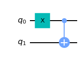
For this example, let’s consider the noise model of a real device ibmq_santiago, and a simple circuit that the output should be $| 11 \rangle$. We would like to do the gate folding of the cx gate, since it is the gate that generates more noise.
import scipy as sp
import numpy as np
import matplotlib.pyplot as plt
import qiskit

from qiskit import QuantumCircuit, transpile, Aer, IBMQ
from qiskit.providers.aer.noise import NoiseModel
from qiskit.utils import QuantumInstance

# Loading your IBM Q account(s)
provider = IBMQ.load_account()
def run_obs(qc, shots, backend_name='ibmq_santiago'):
    """Helper function to get the expected value of the
       | 11 > state.
    """

    # Get device noise model
    device = provider.get_backend(backend_name)
    noise_model = NoiseModel.from_backend(device)
    coupling_map = device.configuration().coupling_map
    seed = 42

    # Define the backend
    backend = QuantumInstance(
                            backend=Aer.get_backend("qasm_simulator"),
                            seed_transpiler=seed,
                            optimization_level=1,
                            noise_model=noise_model,
                            shots=shots,
                            )
    qc = qc.copy()
    qc.measure_all()
    counts = backend.execute(qc).get_counts()
    return counts['11']/shots
qc = QuantumCircuit(2)
qc.x(0)
qc.cx(0, 1)
qc.draw('mpl')
run_obs(qc, 1000)
0.955
In order to fold the circuit in qiskit, we need to create an auxiliary circuit with the folded gates, for this I will base on another tutorial that I did where I showed how to change the gate on an existing circuit.
def fold_cx(qc, alpha):
    """ Fold the cx on the circuit given an alpha value.
    """
    d = qc.depth()
    k = np.ceil(d*(alpha - 1)/2)
    n = k//d
    s = k%d

    instructions = []
    for instruction, qargs, cargs in qc:
        if instruction.name == 'cx':
            instruction = qiskit.circuit.library.CXGate()
            barrier = qiskit.circuit.library.Barrier(len(qc))

            instructions.append((instruction, qargs, cargs))
            instructions.append((barrier, qargs, cargs))
            for _ in range(2*int(n + s)):
                instructions.append((instruction, qargs, cargs))
                instructions.append((barrier, qargs, cargs))


        else:
            instructions.append((instruction, qargs, cargs))

    folded_qc = qc.copy()
    folded_qc.data = instructions
    return folded_qc
Let’s collect the circuit given the alpha value.
alpha_list = [1, 2, 5, 7, 9, 11]
folds = []
for alpha in alpha_list:
    folds.append(fold_cx(qc, alpha))
expected_vals = []
for i in range(len(alpha_list)):
    expected_vals.append(run_obs(folds[i], shots=1000))
print(f"Alphas: {alpha_list}\nExpected values{expected_vals}")
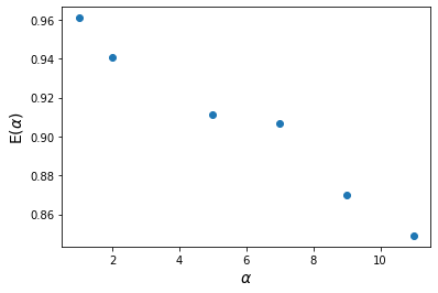
Alphas: [1, 2, 5, 7, 9, 11]
Expected values[0.961, 0.941, 0.911, 0.907, 0.87, 0.849]
plt.plot(alpha_list, expected_vals, 'o')
plt.xlabel(r"$\alpha$", size=14)
plt.ylabel(r"E($\alpha$)", size=14)
plt.show()
Extrapolate E(0)
Now that we’ve colected all $\alpha$ values and $E(\alpha)$ values we can extrapolate the “noiseless” regime. For this case I will use linear extrapolation.
def linear(x, a, b):
    """Linear fit
    """
    return a*x + b

y = expected_vals
x = alpha_list
x, y = np.array(x), np.array(y)

popt, _ = sp.optimize.curve_fit(linear, x, y)
print("Mitigated expectation value:", np.round(popt[1],3))
print("Unmitigated expectation value:", expected_vals[0])
Mitigated expectation value: 0.968
Unmitigated expectation value: 0.961
print("Absolute error with mitigation:", np.round(np.abs(1 - popt[1]), 3))
print("Absolute error without mitigation:", np.round(np.abs(1 - expected_vals[0]), 3))
Absolute error with mitigation: 0.032
Absolute error without mitigation: 0.039
plt.plot(alpha_list, expected_vals, 'o')
plt.plot(0, popt[1], '*', label="mitigated")
plt.xlabel(r"$\alpha$", size=14)
plt.ylabel(r"E($\alpha$)", size=14)
plt.legend()
plt.show()
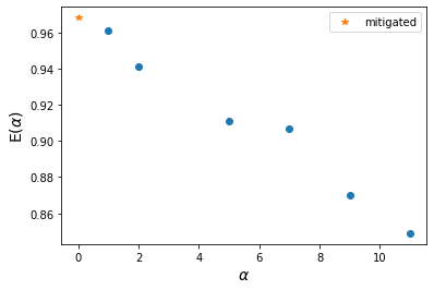
We can see that we got closer to the ideal value of 1, and got a better result than what we would get from the device without error mitigation!
References
[1] - Error mitigation for short-depth quantum circuits - Kristan Temme, Sergey Bravyi, Jay M. Gambetta - Arxiv
[2] - Digital zero noise extrapolation for quantum error mitigation -Tudor Giurgica-Tiron, Yousef Hindy, Ryan LaRose, Andrea Mari, William J. Zeng - Arxiv
Version Information
| Qiskit Software | Version |
|---|---|
| Qiskit | 0.26.2 |
| Terra | 0.17.4 |
| Aer | 0.8.2 |
| Ignis | 0.6.0 |
| Aqua | 0.9.1 |
| IBM Q Provider | 0.13.1 |
| System information | |
| Python | 3.7.5 (default, Feb 23 2021, 13:22:40) [GCC 8.4.0] |
| OS | Linux |
| CPUs | 2 |
| Memory (Gb) | 7.663978576660156 |
| Mon May 31 17:56:11 2021 -03 | |