1) Introduction
Cellular Automaton is a discrete model that can create complex behaviors by using simple rules. The cellular automaton is constructed on a grid with a finite number of states with a deterministic rule for evolution, the surprising fact is that by using a deterministic rule there can be complex behavior that we could not foreseen just by looking on the rule. This model was developed by remarkable people such as Von Neumann, Ulam, Bariccelli. I had contact with this model by Stephen Wolfram’s book A new kind of science. Which is a remarkable, but controversial, book that fascinated me when I was starting in physics at the 2010s.
2) Elementary Cellular Automaton
Cellular Automaton are the simplest kind of program possible, but they present complex behaviors that we cannot predict from the rules alone. This is a recurring theme in nature, simple local rules can give complex global structures. Another remarkable fact is that one rule of the Cellular Automata is Turing Complete, which shows that we can create any computer program by using this rule, showing Turing completeness of this rule is totaly non-trivial, but I refer to the Paper by Matthew Cook that shows this fact. Maybe in the future I will do a post about this proof which I find really beautiful.
2.1) General Rule
Let’s start with the simplest cellular automaton which is 1D with only neighboring interactions (if we have a cell at position i it will only interact with positions i-1 and i+1) and has only two states on and off.
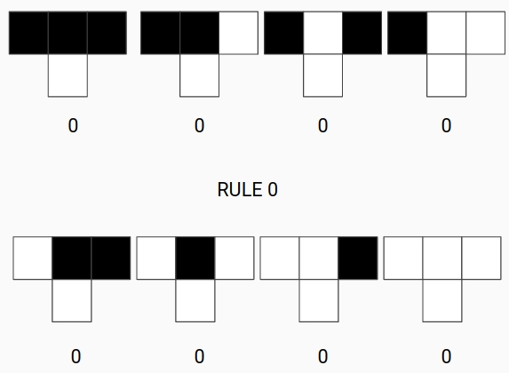
At each iteration we need to give a rule in order to update our array. Each rule needs 3 cells as an input and outputs only one cell, therefore we have $2^3$ possible combinations for each cell can be black or white, thus we have $2^{2^3} = 256$ rules. Since this number can be represented in binary the simplest way to create a rule is to write the number of the rule in binary, this will give the exact output of the rule. As we can see some examples below:
$1_{10} = 00000000_2$
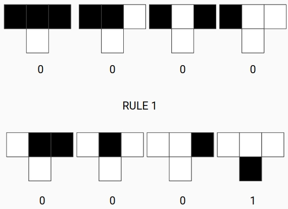
$1_{10} = 00000001_2$
$1_{10} = 00001110_2$
2.2) Taxonomy of Elementary Cellular Automata
Martin, Odlyzko and Wolfram studied all those rules and classified into 4 categories depending on the behavior of random inputs of the rule:
Category I: The Cellular Automata evolves to a stationary state.
Category II: The Cellular Automata evolves into a periodic configuration, each cell has a defined period to return to the original state.
Category III: The Cellular Automata evolves into a periodic configuration.
Category IV: This category collects all Cellular Automata that are not in class I,II, and III.
2.3) Implementation in Python
In this implentation I chose to do with periodic boundary conditions, therefore if you have a cell with in the far right it will be neighbor with the cell in the far left. Let’s walk through the program:
- Convert the rule number into binary and check if the size of this binary is 8, if it is not 8, fill the left values with 0 until it has size eight.
- We use the order defined by Wolfram to map 8-bitstring into the conditions of the Cellular Automaton.
- We set the initial state of the Cellular Automaton
- In this step we do the time evolution of the Cellular Automaton, this is done in three parts:
- 4.1) We ignore the initial state that we put on step 3 skipping the first line.
- 4.2) We run over the 8-bitstring and apply the rule.
def Elementary_Automata(N,T,n,start=None):
    """Function to construct an Elementary Cellular
    automata given by a rule N with periodic Boundary
    Conditions.

    Parameters
    -------------------------------------------------
    N: Rule (int)
    T: Number of steps (int)
    n: Number of the lattice (int)
    start(default = None): Starting Configuration of
                           the lattice. (list)

    Outputs
    -------------------------------------------------
    A: Matrix with the cellular automata evolution
       (np.array)

    """
    # 1)
    #Transform to a bit-string
    N_Bit = bin(N)[2:]

    #Check if the number is an 8-Bit string
    #if not, you add 0 on the right of the string.
    if len(N_Bit)< 8:
        ad = 8 - len(N_Bit)
        aux = ad*'0'
        N_E_Bit = aux + N_Bit

    else:
        N_E_Bit = N_Bit

    # 2)
    # States defined by wolfram
    States = ['111','110','101','100','011','010','001','000']

    #Building a Matrix
    A = np.zeros((T,n))

    # 3)
    #Choose a starting state
    if start == None:
        A[0][np.random.randint(n)] = 1
    else:
        A[0][start] = 1

    # 4)
    for (i,j),_ in np.ndenumerate(A):
        # 4.1)
        if i>0:
            # 4.2)
            for B,S in zip(N_E_Bit,States):
                if (A[i-1][j-1] == int(S[0]) and A[i-1][j] == int(S[1])
                    and A[i-1][(j+1)%n] == int(S[2]) ):
                    A[i][j] = int(B)
    return A
2.4) Examples of Elementary Cellular Automata
Here are some examples:
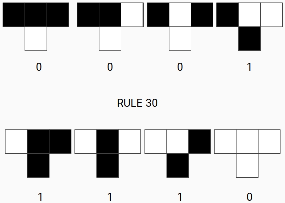
- Rule 30: This rule has been shown to have chaotic behavior and can be used as a random number generator, as it is by the wolfram language:

Rule 30
- Rule 90: This rule produces a fractal that is known as the Sierpinsky Triangle, which comes up when you have the binomial coefficient $\binom{N}{k} \mod 2$. That is, if we construct the Pascal’s Triangle mod 2 we have the Sierpinsky Triangle. This is also known as an additive cellular automaton, because of the relation with mod 2.
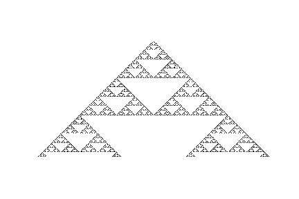
Rule 90
If you want to build your own Elementary Cellular Automaton, the source code for the 1D Cellular Automaton is on github.
References
(1) - Paul Charbonneau - Natural Complexity: A Modeling Handbook